Different approach to Black Scholes model and validation of dynamic delta hedging with Monte Carlo simulation

In my recent article An alternative calculation of the Black Scholes formula for effective hedging programmes, I described d1 and d2 as z-values for two different populations with the same volatility, but two different means.

Viewing the Black-Scholes model in terms of two distributions with different means provides the opportunity to present statistical analysis graphically. This can be particularly advantageous for visually oriented treasurers when utilising the Black-Scholes model. An understanding of option pricing is critical to successful risk management.

In this article, I will show the advantages of understanding of d1 and d2 in the Black-Scholes formula as expressions of two different populations and check whether the dynamic delta hedging survives a test of the Monte Carlo simulation. New technologies combined with analytics and artificial intelligence create opportunities for treasury excellence. I am including in my article a part of my ‘discussion’ with ChatGPT about the meaning of N(d1) and N(d2).

The idea of dynamic delta hedging requires a continuous rebalancing of the portfolio. Dynamic delta hedging is applied by market makers to protect their position. We want to show and check how it works and whether provides promised protection. Hedge fund managers may also apply dynamic hedging to protect their position, we do not suggest that this would be the right strategy for corporate treasurers. The Black Scholes Model is one the most influential ideas in the last 50 years.

Alternative calculation of N(d1) and N(d2)

 mean1 = Logarithm (Spot Price) + (0.5*Volatility^2 + Risk free rate – Dividend)*Time)

mean2 = Logarithm (Spot Price)+ (-0.5*Volatility^2 + Risk free rate – Dividend)*Time)

N(d1) =1 – Lognorm.dist(Strike Price,mean1,Volatility*Time^0.5,True)

N(d2) =1 – Lognorm.dist(Strike Price,mean2,Volatility*Time^0.5,True)

Z-Score is a measurement of how many standard deviations the data point is from the mean of the population and helps to understand where specific data falls within the distribution. Z- table or normal distribution function in Excel gives the probability that the normal random variable will not exceed the value as represented by Z-Score.

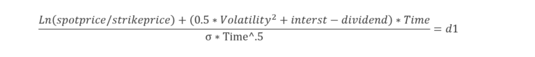
However, in the Black Scholes Model in the case of call options we are interested to know probabilities where stock prices are higher than the strike price, therefore d1 and d2 were multiplied by minus 1 to be able to directly use the Z-table. Therefore, we have to multiply the z-score by minus 1 or use the 1-(Z-table probability).  We can convert Mean 1 into d1 by entering it into z-score formula and multiplying it by minus 1:

 

Now multiply by minus 1

Now just write the logarithm as fraction (negative goes to the denominator)

Many treasurers have calculated d1 and d2 without any thought that they are working with z-values.

The Black-Scholes formula expresses the value of a call option by taking the current stock price discounted by dividend yield multiplied by a probability factor N(d1), and subtracting the exercise price discounted by the risk-free interest rate times a second probability factor N(d2). N is just the notation telling us that we are calculating the probability under the normal distribution curve.

How can we explain what is N(d1) and N(d2)? What is a more beneficial way of looking on Black Scholes formula from the perspective of z-values d1 and d2 or using mean1 and mean2 as I suggest. Which calculation has more meaning or provides a better explanation of what we are doing?

Explaining what d1 and d2 represent can be difficult. The original research papers by Black and Scholes didn’t explain or interpret d1 and d2, and neither did the papers published by Merton. Entire research papers have been written about d1 and d2 alone. According to Lars Tyge Nielsen N(d2) is the risk adjusted probability of exercise – the probability of the asset price exceeding exercise price. “The risk adjusted probability for option exercise is N(d2). It’s linkage to X suggests that it only depends on when the event S_T>X occurs.”

The N(d1) is contingent probability.  N(d1) will always be greater than N(d2). “The expected value of the receipt of the stock is contingent on the exercise of the option. It is, therefore, the product of the conditional expected value of the receipt of S_T given that exercise has occurred times the probability of exercise.” Mathematically the d1 and d2 differ only by volatility times square root of time.

Learning from AI

Black Scholes Model also uses N(d1) as the hedging ratio. Why N(d1) and not N(d2), they just differ by standard deviation times square of time?

Which statement is correct N(d1) is contingent probability and N(d2) a risk adjusted probability or d1 and d2 are z-values for two different populations with the same volatility but two different means. I asked AI to answer this question and had the following chat with Chat GPT:

 

Analysing the Black Scholes Model under the assumption that N(d1) and N(d2) are probabilities of two lognormal distributions with the same standard deviation but different means, gives us the opportunity to interpret Black Scholes model with help of graphical analysis.

In Table 1, we have calculated the Black Scholes call premium for assets with continues return, for example foreign exchange. The traditional calculation shows d1, d2, N(d1), N(d2).  We also calculate Mean 1 and Mean 2.  Already from Graphic 1, we can see if a population has a lower mean, it will have lower probability for the same data than population with higher mean. In the table 1 Mean 1 is 3.29. The mean of the population is the expected or most probable outcome.

When the logarithm of strike price is 3.22 (Ln(25)=3.22), then according to the population with the mean of 3.29, it is 57% probable that asset prices will be higher than ln(25). The probability that stochastic variables under the normal distribution curve are above the mean is 50%. When we start with a variable, which is smaller than mean, then the probability that at maturity prices will be higher is more than 50%, here 57%.

Using Mean 2 we can say that asset prices with probability of 41% will be higher than strike price. Again, here the mean is 3.13 and the logarithm of current stock price equivalent to strike price is above this mean. The probability that prices in this population will be higher than 3.22=ln(25) is only 41%.   Different probabilities of d1 and d2 are not the result of conditional or risk adjusted probabilities but the outcome of applying of two different populations with different means.

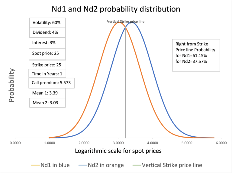
We can also show this with the help of the graphic, see Graphic 2. We use the same data as in table 1. The area links from the vertical strike price line until the orange normal distribution curve, which represents Nd2 amounts to 41.1% and the area links from the vertical strike price line until the blue normal distribution curve, which represents the Nd1 amounts to 56.95%. When we see Nd1 and Nd2 as the two different populations in the Black Scholes Model we can see the impact of changes of various variables.

Higher volatility leads to wider normal distribution. The probability that prices can move higher is bigger and correspondingly option premium rises. However also applied spot and strike price, interest and dividends, respectively foreign interest, lead to changes in the shape of normal distribution. We will show this with the help of the next few graphics.

Graphic 2 and Graphic 3 show the impact of volatility on the shape of the normal distribution curves. In graphic 2 the volatility is 40% and in graphic 3 the volatility is 60%, therefore the graphic 3 normal distribution curves are wider, the probability that spot rates can make bigger swings is higher, also the call premium in graphic 3 is higher. In graphic 4 we show the impact of the increase of interest rate from 3% to 10%. As per formula to calculate the mean of the distribution the 7% difference is added and means increase and both distributions move to the right.

The probability that spot prices will be higher than strike price increases and correspondingly the call premium is higher than in graphic 2. When you check the formulas for mean 1 and mean 2 you notice that dividends or foreign interest will be subtracted. So, if we increase the dividends the distributions curves would move to the left, the probability that spot prices will be higher than strike price goes down and call premium would be lower as well.

Interestingly we could achieve the same movement of the curves to left or right by changing interest or dividends but also by changing the spot price. Instead of increasing the interest rate to 10%, we could change the spot price. Changing the spot price from 25.00 to 26.811 is equivalent to an increase in interest rate from 3% to 10%. The normal distribution curves in graphic 4 and graphic 5 are identical.  The call premiums are not the same. The spot price is different and discounting factor is different, so call premiums must be different as well.

We can discover these interdependencies when we apply graphical analysis not just by calculation of d1 or d2. When you interpret Nd1 and Nd2 as two different distributions you can graphically analyze the impact of each variable in the Black Scholes equation, and this is more meaningful than saying one is risk adjusted and the other contingent probability.

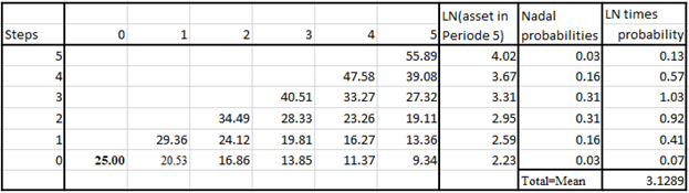
We introduced in our analyzis mean1 and mean2. However the true mean of the population as used when applying binomial trees to calculate option premium, is the mean 2. When creating binomial trees according to to Cox, Ross and Rubinstein method or Jarrow and Rudd method we obatin the mean asset price equal to mean 2.

We see in Table 2 that under assumptions as shown in Table 1 asset prices in the last period, here period 5, reach values which have the mean according to the mean 2. The mean of the distribution according to binomial tree is 3.1289 and this is the mean 2 (derived from d2) in the Black Scholes Model.

We will check with Monte Carlo simulations how good N(d1) as hedging ratio performs and compare this with hedging ratio as per N(d2).  It is very interesting that mean 2 is the true mean of the population created using binomial trees but hedging according to N(d2) is not quite successful.

Simulating asset prices in Excel can be done using various methods, but the most used method is the Monte Carlo simulation. The Monte Carlo simulation is a statistical method used to model the probability of different outcomes in a process that has inherent uncertainty. In the context of asset prices, Monte Carlo simulation can be used to estimate the future prices of financial instruments such as stocks, bonds, foreign exchange, and options.

The Monte Carlo Simulation

The Monte Carlo simulation of asset prices involves using a random number generator to generate many possible future scenarios based on random walk assumption. These scenarios are then used to estimate the distribution of possible future prices of the asset.

We will assume random walk using the following formula:

We implement this in excel using random generator function, table 3 for the basis of our model.

Asset prices are simulated using assumed daily return and daily volatility and using the NORM.INV and RAND functions in Excel to calculate the asset price for the next day. Now we use delta according to N(d1) or N(d2), in Table 3 we are showing N(d2) as dynamic hedge ratio. Comparing delta from the current day to the previous day, we obtain the delta change. Delta change is the amount we must hedge; this means buying or selling accordingly the portion of the asset. In the last column we show hedging costs.

We use the same rate for borrowing and deposit, and can therefore assume that each transaction will last up to the end of the period – in the example, this is 1 year. The first day we purchased 0.4110 assets at the price of 25.  This transaction will generate costs according to the risk-free interest (3%) and provide income according to the dividend yield of 4%, both calculated with continuous compounding. This amounts to 10.17 per period.

The following day, the asset price changes to 25.47 and additional delta hedging must be executed; this would be for a period one day shorter.  All hedging transactions will be added together, plus the amount which we have received as an option premium together with earned interest for the period. At the end of the period, the option will be exercised if the last spot price is higher than the strike price.

The impact of exercise or no exercise must be considered as well. The total amount should be close to zero if the dynamic hedging is a perfect hedging as Black Scholes Model assumes. In Table 5, the difference between received premium plus interest, versus synthetic premium obtained through delta hedging, is shown as ‘Result of sim’.  Any simulation can provide different results.

We used an Excel data table to repeat each year, 1000 times.  Instead of a premium of $ 3.71, as per Black Scholes, with dynamic hedging we would get $3.7127 – a  difference of $0.0027.

$0.0027 is the average difference of many simulations. The maximum difference (repeating each year, 1000 times with the data table) provides a difference of $0.5023.

In any individual year the results of delta hedging simulation can deviate from the Black Scholes model value by some 15% to 25%. However, when performing many simulations, they converge to the theoretical value as predicted by Black Scholes model.  The practical message for the treasurer is, you cannot rely on dynamic delta hedging when you apply it sporadically. Dynamic delta hedging is an instrument which can be used by market makers when applied on continuous basis; then they can assume that on average results can be as predicted by the model.

Dynamic hedging success hinges on volatility

With the help of the VBA we have repeated this exercise 500 times and calculated the final average results, which are now shown in Table 5 and represent an average result of 130 million simulations for each case.

The row with a description ‘Result of sim’ shows the deviation from the Black Scholes premium. In the first simulation (upper left corner), 0.004 means the dynamic hedging costs were $0.004 lower than option premium according to the Black Scholes model. With dynamic hedging, we obtained 0.11% more than we charged for the call premium.

The whole analysis assumed no transactions costs and no bid/offer spread. We simulated for money options various returns from -20% to +25% p.a.  We also checked money in and out of the money options. As long the volatility remains as implied volatility in the Black Scholes model, the dynamic delta hedging according to N(d1) shows almost perfect results. When we change volatility dynamic hedging does not provide sufficient protection.

When volatility goes down, we will achieve much better results, but when volatility goes up the results deteriorate substantially and the dynamic delta hedging according to N(d1) does not provide sufficient protection.  When we use N(d2) as the delta ratio for dynamic delta hedging, we cannot speak about hedging but more about speculation. When you check the results in Table 5, you see that delta based on N(d2) rarely show better results. Only when we assume substantial negative return, “hedging” as per N(d2) shows substantial positive results.

However, underperformance under return of +20% is higher than positive performance using return of-20%, -11.43% versus 9.45% for at the money options at 40% volatility.

If we knew that a particular asset will perform negatively in the future, we can contemplate applying delta hedging according to N(d2), but in my view this would be speculation rather than hedging. Treasurers who plan to create synthetic options using dynamic hedging must keep in mind that they are exposed to high volatility risk and must seek to hedge volatility.

Vega hedging might be a potential remedy. Vega hedging is a method of managing risk by establishing a hedge against the implied volatility used in the Black Scholes model. By Vega hedging an options position, treasurer can reduce the risk associated with changes in implied volatility and make the portfolio more stable. However, Vega hedging can be complex and requires a deep understanding of options trading and risk management techniques. Vega hedging can also be checked using the Monte Carlo simulation, and this might be the topic for a future article.